Research Methods

Modeling in Scientific Research

LEGO® bricks have been a staple of the toy world since they were first manufactured in Denmark in 1953. The interlocking plastic bricks can be assembled into an endless variety of objects (see Figure 1). Some kids (and even many adults) are interested in building the perfect model – finding the bricks of the right color, shape, and size, and assembling them into a replica of a familiar object in the real world, like a castle, the space shuttle, or London Bridge. Others focus on using the object they build – moving LEGO knights in and out of the castle shown in Figure 1, for example, or enacting a space shuttle mission to Mars. Still others may have no particular end product in mind when they start snapping bricks together and just want to see what they can do with the pieces they have.

On the most basic level, scientists use models in much the same way that people play with LEGO bricks. Scientific models may or may not be physical entities, but scientists build them for the same variety of reasons: to replicate systems in the real world through simplification, to perform an experiment that cannot be done in the real world, or to assemble several known ideas into a coherent whole to build and test hypotheses.

Types of models: Physical, conceptual, mathematical

At the St. Anthony Falls Laboratory at the University of Minnesota, a group of engineers and geologists have built a room-sized physical replica of a river delta to model a real one like the Mississippi River delta in the Gulf of Mexico (Paola et al., 2001). These researchers have successfully incorporated into their model the key processes that control river deltas (like the variability of water flow, the deposition of sediments transported by the river, and the compaction and subsidence of the coastline under the pressure of constant sediment additions) in order to better understand how those processes interact. With their physical model, they can mimic the general setting of the Mississippi River delta and then do things they can't do in the real world, like take a slice through the resulting sedimentary deposits to analyze the layers within the sediments. Or they can experiment with changing parameters like sea level and sedimentary input to see how those changes affect deposition of sediments within the delta, the same way you might "experiment" with the placement of the knights in your LEGO castle.

Not all models used in scientific research are physical models. Some are conceptual, and involve assembling all of the known components of a system into a coherent whole. This is a little like building an abstract sculpture out of LEGO bricks rather than building a castle. For example, over the past several hundred years, scientists have developed a series of models for the structure of an atom. The earliest known model of the atom compared it to a billiard ball, reflecting what scientists knew at the time – they were the smallest piece of an element that maintained the properties of that element. Despite the fact that this was a purely conceptual model, it could be used to predict some of the behavior that atoms exhibit. However, it did not explain all of the properties of atoms accurately. With the discovery of subatomic particles like the proton and electron, the physicist Ernest Rutherford proposed a "solar system" model of the atom, in which electrons orbited around a nucleus that included protons (see our Atomic Theory I: The Early Days module for more information). While the Rutherford model is useful for understanding basic properties of atoms, it eventually proved insufficient to explain all of the behavior of atoms. The current quantum model of the atom depicts electrons not as pure particles, but as having the properties of both particles and waves, and these electrons are located in specific probability density clouds around the atom's nucleus.

Both physical and conceptual models continue to be important components of scientific research. In addition, many scientists now build models mathematically through computer programming. These computer-based models serve many of the same purposes as physical models, but are determined entirely by mathematical relationships between variables that are defined numerically. The mathematical relationships are kind of like individual LEGO bricks: They are basic building blocks that can be assembled in many different ways. In this case, the building blocks are fundamental concepts and theories like the mathematical description of turbulent flow in a liquid, the law of conservation of energy, or the laws of thermodynamics, which can be assembled into a wide variety of models for, say, the flow of contaminants released into a groundwater reservoir or for global climate change.

Modeling as a scientific research method

Whether developing a conceptual model like the atomic model, a physical model like a miniature river delta, or a computer model like a global climate model, the first step is to define the system that is to be modeled and the goals for the model. "System" is a generic term that can apply to something very small (like a single atom), something very large (like the Earth's atmosphere), or something in between, like the distribution of nutrients in a local stream. So defining the system generally involves drawing the boundaries (literally or figuratively) around what you want to model, and then determining the key variables and the relationships between those variables.

Though this initial step may seem straightforward, it can be quite complicated. Inevitably, there are many more variables within a system than can be realistically included in a model, so scientists need to simplify. To do this, they make assumptions about which variables are most important. In building a physical model of a river delta, for example, the scientists made the assumption that biological processes like burrowing clams were not important to the large-scale structure of the delta, even though they are clearly a component of the real system.

Determining where simplification is appropriate takes a detailed understanding of the real system – and in fact, sometimes models are used to help determine exactly which aspects of the system can be simplified. For example, the scientists who built the model of the river delta did not incorporate burrowing clams into their model because they knew from experience that they would not affect the overall layering of sediments within the delta. On the other hand, they were aware that vegetation strongly affects the shape of the river channel (and thus the distribution of sediments), and therefore conducted an experiment to determine the nature of the relationship between vegetation density and river channel shape (Gran & Paola, 2001).

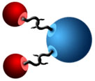
Once a model is built (either in concept, physical space, or in a computer), it can be tested using a given set of conditions. The results of these tests can then be compared against reality in order to validate the model. In other words, how well does the model do at matching what we see in the real world? In the physical model of delta sediments, the scientists who built the model looked for features like the layering of sand that they have seen in the real world. If the model shows something really different than what the scientists expect, the relationships between variables may need to be redefined or the scientists may have oversimplified the system. Then the model is revised, improved, tested again, and compared to observations again in an ongoing, iterative process. For example, the conceptual "billiard ball" model of the atom used in the early 1800s worked for some aspects of the behavior of gases, but when that hypothesis was tested for chemical reactions, it didn't do a good job of explaining how they occur – billiard balls do not normally interact with one another. John Dalton envisioned a revision of the model in which he added "hooks" to the billiard ball model to account for the fact that atoms could join together in reactions, as conceptualized in Figure 3.

While conceptual and physical models have long been a component of all scientific disciplines, computer-based modeling is a more recent development, and one that is frequently misunderstood. Computer models are based on exactly the same principles as conceptual and physical models, however, and they take advantage of relatively recent advances in computing power to mimic real systems.

The beginning of computer modeling: Numerical weather prediction

In the late 19th century, Vilhelm Bjerknes, a Norwegian mathematician and physicist, became interested in deriving equations that govern the large-scale motion of air in the atmosphere. Importantly, he recognized that circulation was the result not just of thermodynamic properties (like the tendency of hot air to rise), but of hydrodynamic properties as well, which describe the behavior of fluid flow. Through his work, he developed an equation that described the physical processes involved in atmospheric circulation, which he published in 1897. The complexity of the equation reflected the complexity of the atmosphere, and Bjerknes was able to use it to describe why weather fronts develop and move.

Using calculations predictively

Bjerknes had another vision for his mathematical work, however: He wanted to predict the weather. The goal of weather prediction, he realized, is not to know the paths of individual air molecules over time, but to provide the public with "average values over large areas and long periods of time." Because his equation was based on physical principles, he saw that by entering the present values of atmospheric variables like air pressure and temperature, he could solve it to predict the air pressure and temperature at some time in the future. In 1904, Bjerknes published a short paper describing what he called "the principle of predictive meteorology" (Bjerknes, 1904) (see the Research links for the entire paper). In it, he says:

Based upon the observations that have been made, the initial state of the atmosphere is represented by a number of charts which give the distribution of seven variables from level to level in the atmosphere. With these charts as the starting point, new charts of a similar kind are to be drawn, which represent the new state from hour to hour.

In other words, Bjerknes envisioned drawing a series of weather charts for the future based on using known quantities and physical principles. He proposed that solving the complex equation could be made more manageable by breaking it down into a series of smaller, sequential calculations, where the results of one calculation are used as input for the next. As a simple example, imagine predicting traffic patterns in your neighborhood. You start by drawing a map of your neighborhood showing the location, speed, and direction of every car within a square mile. Using these parameters, you then calculate where all of those cars are one minute later. Then again after a second minute. Your calculations will likely look pretty good after the first minute. After the second, third, and fourth minutes, however, they begin to become less accurate. Other factors you had not included in your calculations begin to exert an influence, like where the person driving the car wants to go, the right- or left-hand turns that they make, delays at traffic lights and stop signs, and how many new drivers have entered the roads.

Trying to include all of this information simultaneously would be mathematically difficult, so, as proposed by Bjerknes, the problem can be solved with sequential calculations. To do this, you would take the first step as described above: Use location, speed, and direction to calculate where all the cars are after one minute. Next, you would use the information on right- and left-hand turn frequency to calculate changes in direction, and then you would use information on traffic light delays and new traffic to calculate changes in speed. After these three steps are done, you would solve your first equation again for the second minute time sequence, using location, speed, and direction to calculate where the cars are after the second minute. Though it would certainly be rather tiresome to do by hand, this series of sequential calculations would provide a manageable way to estimate traffic patterns over time.

Although this method made calculations tedious, Bjerknes imagined "no intractable mathematical difficulties" with predicting the weather. The method he proposed (but never used himself) became known as numerical weather prediction, and it represents one of the first approaches towards numerical modeling of a complex, dynamic system.

Advancing weather calculations

Bjerknes' challenge for numerical weather prediction was taken up sixteen years later in 1922 by the English scientist Lewis Fry Richardson. Richardson related seven differential equations that built on Bjerknes' atmospheric circulation equation to include additional atmospheric processes. One of Richardson's great contributions to mathematical modeling was to solve the equations for boxes within a grid; he divided the atmosphere over Germany into 25 squares that corresponded with available weather station data (see Figure 4) and then divided the atmosphere into five layers, creating a three-dimensional grid of 125 boxes. This was the first use of a technique that is now standard in many types of modeling. For each box, he calculated each of nine variables in seven equations for a single time step of three hours. This was not a simple sequential calculation, however, since the values in each box depended on the values in the adjacent boxes, in part because the air in each box does not simply stay there – it moves from box to box.

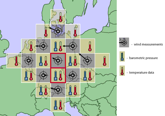
Richardson's attempt to make a six-hour forecast took him nearly six weeks of work with pencil and paper and was considered an utter failure, as it resulted in calculated barometric pressures that exceeded any historically measured value (Dalmedico, 2001). Probably influenced by Bjerknes, Richardson attributed the failure to inaccurate input data, whose errors were magnified through successive calculations (see more about error propagation in our Uncertainty, Error, and Confidence module).

In addition to his concerns about inaccurate input parameters, Richardson realized that weather prediction was limited in large part by the speed at which individuals could calculate by hand. He thus envisioned a "forecast factory," in which thousands of people would each complete one small part of the necessary calculations for rapid weather forecasting.

First computer for weather prediction

Richardson's vision became reality in a sense with the birth of the computer, which was able to do calculations far faster and with fewer errors than humans. The computer used for the first one-day weather prediction in 1950, nicknamed ENIAC (Electronic Numerical Integrator and Computer), was 8 feet tall, 3 feet wide, and 100 feet long – a behemoth by modern standards, but it was so much faster than Richardson's hand calculations that by 1955, meteorologists were using it to make forecasts twice a day (Weart, 2003). Over time, the accuracy of the forecasts increased as better data became available over the entire globe through radar technology and, eventually, satellites.

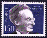
The process of numerical weather prediction developed by Bjerknes and Richardson laid the foundation not only for modern meteorology, but for computer-based mathematical modeling as we know it today. In fact, after Bjerknes died in 1951, the Norwegian government recognized the importance of his contributions to the science of meteorology by issuing a stamp bearing his portrait in 1962 (Figure 5).

Modeling in practice: The development of global climate models

The desire to model Earth's climate on a long-term, global scale grew naturally out of numerical weather prediction. The goal was to use equations to describe atmospheric circulation in order to understand not just tomorrow's weather, but large-scale patterns in global climate, including dynamic features like the jet stream and major climatic shifts over time like ice ages. Initially, scientists were hindered in the development of valid models by three things: a lack of data from the more inaccessible components of the system like the upper atmosphere, the sheer complexity of a system that involved so many interacting components, and limited computing powers. Unexpectedly, World War II helped solve one problem as the newly-developed technology of high altitude aircraft offered a window into the upper atmosphere (see our Technology module for more information on the development of aircraft). The jet stream, now a familiar feature of the weather broadcast on the news, was in fact first documented by American bombers flying westward to Japan.

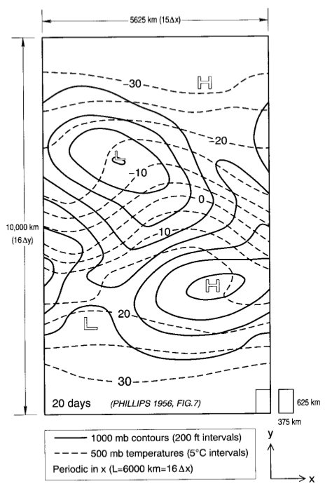
As a result, global atmospheric models began to feel more within reach. In the early 1950s, Norman Phillips, a meteorologist at Princeton University, built a mathematical model of the atmosphere based on fundamental thermodynamic equations (Phillips, 1956). He defined 26 variables related through 47 equations, which described things like evaporation from Earth's surface, the rotation of the Earth, and the change in air pressure with temperature. In the model, each of the 26 variables was calculated in each square of a 16 x 17 grid that represented a piece of the northern hemisphere. The grid represented an extremely simple landscape – it had no continents or oceans, no mountain ranges or topography at all. This was not because Phillips thought it was an accurate representation of reality, but because it simplified the calculations. He started his model with the atmosphere "at rest," with no predetermined air movement, and with yearly averages of input parameters like air temperature.

Phillips ran the model through 26 simulated day-night cycles by using the same kind of sequential calculations Bjerknes proposed. Within only one "day," a pattern in atmospheric pressure developed that strongly resembled the typical weather systems of the portion of the northern hemisphere he was modeling (see Figure 6). In other words, despite the simplicity of the model, Phillips was able to reproduce key features of atmospheric circulation, showing that the topography of the Earth was not of primary importance in atmospheric circulation. His work laid the foundation for an entire subdiscipline within climate science: development and refinement of General Circulation Models (GCMs).

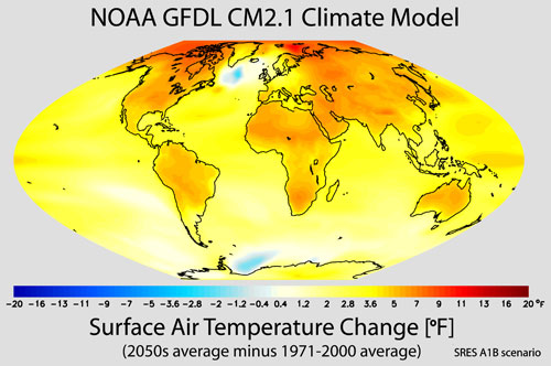
By the 1980s, computing power had increased to the point where modelers could incorporate the distribution of oceans and continents into their models. In 1991, the eruption of Mt. Pinatubo in the Philippines provided a natural experiment: How would the addition of a significant volume of sulfuric acid, carbon dioxide, and volcanic ash affect global climate? In the aftermath of the eruption, descriptive methods (see our Description in Scientific Research module) were used to document its effect on global climate: Worldwide measurements of sulfuric acid and other components were taken, along with the usual air temperature measurements. Scientists could see that the large eruption had affected climate, and they quantified the extent to which it had done so. This provided a perfect test for the GCMs. Given the inputs from the eruption, could they accurately reproduce the effects that descriptive research had shown? Within a few years, scientists had demonstrated that GCMs could indeed reproduce the climatic effects induced by the eruption, and confidence in the abilities of GCMs to provide reasonable scenarios for future climate change grew. The validity of these models has been further substantiated by their ability to simulate past events, like ice ages, and the agreement of many different models on the range of possibilities for warming in the future, one of which is shown in Figure 7.

Limitations and misconceptions of models

The widespread use of modeling has also led to widespread misconceptions about models, particularly with respect to their ability to predict. Some models are widely used for prediction, such as weather and streamflow forecasts, yet we know that weather forecasts are often wrong. Modeling still cannot predict exactly what will happen to the Earth's climate, but it can help us see the range of possibilities with a given set of changes. For example, many scientists have modeled what might happen to average global temperatures if the concentration of carbon dioxide (CO2) in the atmosphere is doubled from pre-industrial levels (pre-1950); though individual models differ in exact output, they all fall in the range of an increase of 2-6° C (IPCC, 2007).

All models are also limited by the availability of data from the real system. As the amount of data from a system increases, so will the accuracy of the model. For climate modeling, that is why scientists continue to gather data about climate in the geologic past and monitor things like ocean temperatures with satellites – all those data help define parameters within the model. The same is true of physical and conceptual models, too, well-illustrated by the evolution of our model of the atom as our knowledge about subatomic particles increased.

Modeling in modern practice

The various types of modeling play important roles in virtually every scientific discipline, from ecology to analytical chemistry and from population dynamics to geology. Physical models such as the river delta take advantage of cutting edge technology to integrate multiple large-scale processes. As computer processing speed and power have increased, so has the ability to run models on them. From the room-sized ENIAC in the 1950s to the closet-sized Cray supercomputer in the 1980s to today's laptop, processing speed has increased over a million-fold, allowing scientists to run models on their own computers rather than booking time on one of only a few supercomputers in the world. Our conceptual models continue to evolve, and one of the more recent theories in theoretical physics digs even deeper into the structure of the atom to propose that what we once thought were the most fundamental particles – quarks – are in fact composed of vibrating filaments, or strings. String theory is a complex conceptual model that may help explain gravitational force in a way that has not been done before. Modeling has also moved out of the realm of science into recreation, and many computer games like SimCity® involve both conceptual modeling (answering the question, "What would it be like to run a city?") and computer modeling, using the same kinds of equations that are used model traffic flow patterns in real cities. The accessibility of modeling as a research method allows it to be easily combined with other scientific research methods, and scientists often incorporate modeling into experimental, descriptive, and comparative studies.

Summary

Scientific modeling is a research method scientists use to replicate real-world systems 0 whether it's a conceptual model of an atom, a physical model of a river delta, or a computer model of global climate. This module describes the principles that scientists use when building models and shows how modeling contributes to the process of science.

Key Concepts

• Modeling involves developing physical, conceptual, or computer-based representations of systems.
• Scientists build models to replicate systems in the real world through simplification, to perform an experiment that cannot be done in the real world, or to assemble several known ideas into a coherent whole to build and test hypotheses.
• Computer modeling is a relatively new scientific research method, but it is based on the same principles as physical and conceptual modeling.

QUIZ

1. In order to provide realistic output, scientific models

(A)__incorporate all known variables in the real world.

(B)__must be accurate representations of a system.

(C)__use equations to describe every process within a system.

(D)__simplify the real world where appropriate.

2. Vilhelm Bjerknes saw "no intractable mathematical difficulties" with predicting the weather, and many numerical models have been built since he wrote those words in 1904. Even with the best of those models, our weather predictions are still frequently incorrect. Why?

(A)__Bjerknes was wrong: The math is too complicated.

(B)__Not all aspects of weather can be described mathematically.

(C)__We don't have fast enough computers to do the calculations in time.

(D)__The weather system is very complex: Small changes in variables can have big effects.

3. Why is climate particularly well suited to research using modeling rather than other methods like experimentation?

(A)__We know all of the equations describing air circulation in the atmosphere.

(B)__Modeling allows us to study the effect of changes in a complex system.

(C)__It is impossible to do experiments in climate science.

(D)__We don't have another system with which to compare Earth's climate.

4. Hydrologists have developed a computer-based model to simulate flow of a contaminant through a groundwater reservoir. In order to develop their model, the hydrologists most likely

(A)__collected data from the reservoir they are modeling.

(B)__took an existing groundwater model and modified it to suit their needs.

(C)__simplified the shape of the reservoir in the model.

(D)__did all of the things listed as answers.

5. Physical "ball-and-stick" models are often used to represent molecules, even though scientists agree that atoms are not like billiard balls and bonds are not like sticks holding them together. Why do you think these are still used?

(A)__Scientists haven't been able to come up with a better model.

(B)__Better models are available, but ball and stick models are easy to create and explain.

(C)__For some purposes, such as visualizing spatial relationships, the model is useful.

(D)__all of these answers are correct.

6. The first step a scientist takes in developing a model - conceptual, numerical, or physical - is to define the system that the model is meant to represent. Which of the following statements best describe a system?

   (A)__A system has boundaries defined by a researcher.

   (B)__A system in a model should not simplify a real system.

   (C)__A system includes many variables, all of which are equally important.

   (D)__A system is a large entity with many variables and processes.

7. Computer models are superior to physical models because they are more quantitative.

(A)__true

(B)__false